Contents
INTRODUCTION
Original Author: Damiano Vitulli
Translation by: Click here
Vectors and normals... great words! Certainly, most of you would have come across these at school during either physics or geometry. But, you would never have imagined that one day you would have use these notions to create a 3d engine! Anyway, don't worry too much, you won't have to re-open your old dusty books! In this lesson we will cover vectors in detail, and we will program a library to manage them.
The first practical application of vectors deals with the calculations relating to illumination within the world. Many of you could be wondering why we need to bother with this because it's clear that the scene is already uniformly illuminated! Why we need to insert lights then?
Until now we have drawn our virtual world using a uniform, non-realistic illumination. Illuminating objects means drawing them with shiny and shaded parts, which shows more accurately what the object would look like in the real world. Disorder and chaos are the keywords you should keep in mind for your 3d engine. But please, your source code has to be ordered and clear as well =)
With this lesson we will increase the realism of our virtual world.
FUNDAMENTAL NOTIONS ON STRAIGHT LINES, VECTORS and NORMALS
Ok guys, now we have to face up to some theory. Keep in mind that all we are going to study is what is essential to perform the calculations concerning illumination. So again, take your favourite programming drink and get ready!
Do you know what straight lines and segments are? I hope so. Here is a brief explanation of the the fundamentals anyway:
STRAIGHT LINE
A Straight Line is an endless line, it doesn't have origin, nor an end, but it has a direction. It can be represented by the simple equation y=ax+b.
Two straight lines that have the same direction are called Parallel Straight Lines.
Two straight lines that form an angle of 90 degrees are called Perpendicular Straight Lines.
SEGMENT
If we take two points A and B belonging to a Straight Line, the space included between them is called a Segment. To represent a Segment we often put a hyphen over the two letters: ![]() .
.
The points A and B can run in two possible ways: from A toward B, or from B toward A. A Segment with an assigned orientation is called Oriented Segment and it is represented by putting an arrow over the two extreme points: ![]() .
.
VECTOR
Finally here is the definition of a vector:
(1) A Vector is a quantity that represents every line segment with the same magnitude and the same direction.
This means that two vectors are equal if they have the same direction and the same length, regardless of whether they have the same initial points. That was a geometric definition of a vector, and doesn't really show us the true utility of a vector.
The concept of a vector finds its origins in the field of physics. There are some magnitudes that can be measured simply using a number, these are called Scalar Quantities (i.e. room temperature or mass) Other magnitudes however, like speed or force, have an oriented direction (direction and angle) as well as a numerical component (that can be only positive). These magnitudes are called Vectors.
Graphically a Vector is represented as an arrow, this defines the direction. The length of the arrow represents the numerical component, or Magnitude.
To identify a vector different notations are used.
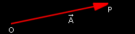
- If we identify the origin of a vector as the point O and the end as the point P, algebraically we can identify the vector using its extreme points: OP.
- The notation more commonly used is a capital letter with an arrow over it, example:

The numerical component, or magnitude, of a vector (its length) is represented using the absolute value sign: magnitude of ![]() =
= ![]()
The last important definition is the Versor:
VERSOR
A versor is a vector with magnitude equal to 1. Often in our 3d engine we will need to transform some vectors into versors, this operation is called: normalizing a vector.
To identify a versor we will use a lower case letter with an arrow over it, example: ![]()
VECTORS IN DETAIL
Now let's begin to organize our data structures to manage these strange vectors! The best thing do when adding a particular functionality to the graphic engine is create a special library, so as to make the code as clean as possible. Therefore we add two blank files: mat_vect.cpp and the relative header mat_vect.h into our development environment. I have decided to insert the prefix "mat" just to identify these as mathematical libraries.
Please have a look at this picture:
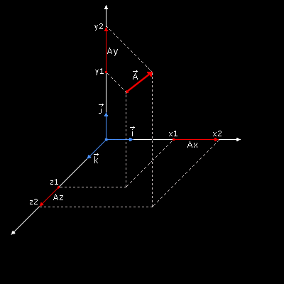
We have split our vector into three vectors that are parallel to the x, y and z axis . Now we can represent the vector using this notation:
(2) ![]() = [(x2-x1),(y2-y1),(z2-z1)]
= [(x2-x1),(y2-y1),(z2-z1)]
And then:
(3) ![]() = (Ax,Ay,Az)
= (Ax,Ay,Az)
This is called the Cartesian Representation of a vector.
Another way to represent a vector is:
(4) ![]() = Ax
= Ax![]() +Ay
+Ay![]() +Az
+Az![]()
where ![]() ,
, ![]() ,
, ![]() are the axis versors.
are the axis versors.
And finally here is a little bit of code, using (3) let's create our vector structure:
typedef struct
{
    float x,y,z;
} p3d_type, *p3d_ptr_type;
We have identified the vector type as a simple 3d point, why? Well, we have simplified the job because by using (1) we can consider all vectors starting from origin. ;-)
CREATION, NORMALIZATION AND LENGTH CALCULATION
To create a vector we use formula (2), we write a function with three parameters: the start point, the end point and the final vector. All the parameters are pointers:
void VectCreate (p3d_ptr_type p_start, p3d_ptr_type p_end, p3d_ptr_type p_vector)
{
    p_vector->x = p_end->x - p_start->x;
    p_vector->y = p_end->y - p_start->y;
    p_vector->z = p_end->z - p_start->z;
    VectNormalize(p_vector);
}
Don't worry now about the function VectNormalize, that I will explain this in a moment.
To calculate the length of a vector (the magnitude) we have to use Pythagoras' Theorem twice, and don't come here saying that you don't remember that theorem! Here is a brief recap if you have forgotten it though:
if we take a right-angle triangle (a triangle with an angle of 90°) the square built on the hypotenuse is equal to the sum of the squares built on the other two sides.
Now its time to use your imagination... have a look at this picture, we have created a vector that starts from the origin of the axis:
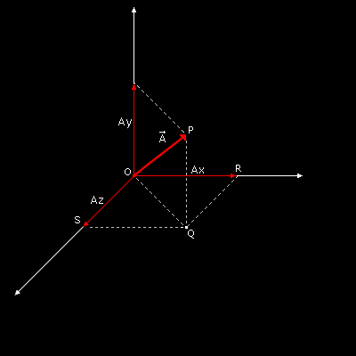
To find the length of the vector ![]() , also called magnitude
, also called magnitude ![]() = OP, we apply the Pythagoras's Theorem to the triangle OPQ:
= OP, we apply the Pythagoras's Theorem to the triangle OPQ:
OP = Square root of (Ay*Ay + OQ*OQ)
Now Ay is known, to calculate OQ we have to apply Pythagoras's Theorem again, this time using the triangle OQR:
OQ*OQ = (Ax*Ax + Az*Az)
We fill this expression into the first equation and we find the length (magnitude) of the vector:
OP = Square root of (Ax*Ax + Ay*Ay + Az*Az)
And here is the function in C:
float VectLenght (p3d_ptr_type p_vector)
{
    return (float)(sqrt(p_vector->x*p_vector->x + p_vector->y*p_vector->y + p_vector->z*p_vector->z));
}
We have already said that normalizing a vector means transforming its length to 1. To do this we divide all the vector's components: Ax, Ay, Az by its length (magnitude).
void VectNormalize(p3d_ptr_type p_vector)
{
    float l_lenght;

    l_lenght = VectLenght(p_vector);
    if (l_lenght==0) l_lenght=1;
    p_vector->x /= l_lenght;
    p_vector->y /= l_lenght;
    p_vector->z /= l_lenght;
}
SUM AND DIFFERENCE
There are 4 fundamental operations that we can do with vectors: sum, difference, scalar product and vector product.
The sum of two vectors ![]() and
and ![]() is another vector
is another vector ![]() , which is obtained by applying the vertex of
, which is obtained by applying the vertex of ![]() the origin of
the origin of ![]() and connecting with a line the origin of
and connecting with a line the origin of ![]() to the end of
to the end of ![]() .
.
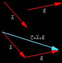
If we represent the two vectors using the notation (3) then the sum of two vectors can be obtained also using the analytical method:
![]() +
+ ![]() = (Ax + Bx, Ay + By, Az + Bz)
= (Ax + Bx, Ay + By, Az + Bz)
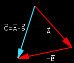
The difference of two vectors is a particular case of the sum and it is obtained applying to the vertex of ![]() the origin of -
the origin of -![]() and connecting with a line the origin of
and connecting with a line the origin of ![]() with the end of -
with the end of -![]() .
.
We won't create special functions for the sum and the difference of vectors because there are not useful for now.
SCALAR PRODUCT (OR DOT PRODUCT)
We have two ways to multiply vectors:
- the first one is called scalar product (or dot product) whose result is a simple number.
- the second one is vector product (or cross product) whose result is a vector.
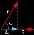
The scalar product is defined as the product of the magnitudes of the vectors times the cosine of the angle between them
![]() dot
dot ![]() =
= ![]() *
* ![]() * cos (
* cos (![]() )
)
This is a geometrical approach that doesn't fit easily in with our source code. We must find a way to express this definition in an analytical approach, so listen:
Using our last definition it is easy to reach these relationships for the axes versors:
(5) ![]() dot
dot ![]() =
= ![]() dot
dot ![]() =
= ![]() dot
dot ![]() = 1
= 1
(6) ![]() dot
dot ![]() =
= ![]() dot
dot ![]() =
= ![]() dot
dot ![]() = 0
= 0
Now let's define two vectors using the definition (4):
![]() = Ax
= Ax![]() + Ay
+ Ay![]() + Az
+ Az![]()
![]() = Bx
= Bx![]() + By
+ By![]() + Bz
+ Bz![]()
And calculate the scalar product:
![]() dot
dot ![]() = (Ax
= (Ax![]() + Ay
+ Ay![]() + Az
+ Az![]() ) dot (Bx
) dot (Bx![]() + By
+ By![]() + Bz
+ Bz![]() )
)
Using the (5) and the (6) we can obtain the scalar product analytic formula.
![]() dot
dot ![]() = Ax*Bx + Ay*By + Az*Bz
= Ax*Bx + Ay*By + Az*Bz
And now let's create the function VectScalarProduct:
float VectScalarProduct (p3d_ptr_type p_vector1,p3d_ptr_type p_vector2)
{
    return (p_vector1->x*p_vector2->x + p_vector1->y*p_vector2->y + p_vector1->z*p_vector2->z);
}
Wow! It's just crazy!
VECTOR PRODUCT (OR CROSS PRODUCT)
After all these notions you will certainly wonder why we are studying all this theory... but be patient be guys, it will all come together when we get to "illumination" =)
Finally, here is the vector product...
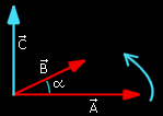
The vector product of two vectors, ![]() and
and ![]() , is defined as another vector
, is defined as another vector ![]() which is calculated in this way:
which is calculated in this way:
- Its magnitude is the product of the magnitudes of vectors and
 multiplied by the sine of the angle between them,
  = x = AB sin(
 ).
).
- Its direction is perpendicular to the plane formed by and and oriented so that a right-handed rotation about it carries into through an angle not greater than 180°.
As we have already done for the scalar product we must find the analytical approach to the vector product, so let's write some relationships:
(7) ![]() x
x ![]() =
= ![]() x
x ![]() =
= ![]() x
x ![]() = 0
= 0
(8) ![]() x
x ![]() =
= ![]()
![]() x
x ![]() =
= ![]()
![]() x
x ![]() =
= ![]()
We now express the two vectors using definition (4):
![]() = Ax
= Ax![]() + Ay
+ Ay![]() + Az
+ Az![]()
![]() = Bx
= Bx![]() + By
+ By![]() + Bz
+ Bz![]()
![]() x
x ![]() = (Ax
= (Ax![]() + Ay
+ Ay![]() + Az
+ Az![]() ) x (Bx
) x (Bx![]() + By
+ By![]() + Bz
+ Bz![]() )
)
After a few steps using (7) and (8) we can obtain the expression of the vector product:
![]() x
x ![]() = (AyBz - AzBy)
= (AyBz - AzBy)![]() + (AzBx - AxBz)
+ (AzBx - AxBz)![]() + (AxBy - AyBx)
+ (AxBy - AyBx)![]()
Finally let's create the function VectDotProduct:
void VectDotProduct (p3d_ptr_type p_vector1,p3d_ptr_type p_vector2,p3d_ptr_type p_vector3)
{
    p_vector3->x=(p_vector1->y * p_vector2->z) - (p_vector1->z * p_vector2->y);
    p_vector3->y=(p_vector1->z * p_vector2->x) - (p_vector1->x * p_vector2->z);
    p_vector3->z=(p_vector1->x * p_vector2->y) - (p_vector1->y * p_vector2->x);
}
That was like an university lecture, don't you think? Now let's relax a little bit, because we are going to switch on the lights. =D
LET'S ILLUMINATE OUR VIRTUAL WORLD
These are the main steps to illuminate our virtual world:
- First of all it is necessary to define and to activate at least one light source in the space.
- For each polygon we need to determine the amount of light that it is able to reflect and to transmit to the eye of our observer.
- In the rendering phase we paint the polygons according to their illumination value.
We will now analyze these various points in detail.
LIGHT POINTS DEFINITION AND ACTIVATION
To implement the illumination there are two main elements to consider: the light source and the material properties.
OpenGL considers the light constituted by 3 fundamental components: ambient, diffuse and specular.
- The Ambient component is the light whose direction is impossible to be determined since it seems to come from all directions. It is mainly light that has been reflected several times. A polygon is always uniformly illuminated by the ambient environment, it doesn't matter what orientation or position it has in the space.
- The Diffuse component is the light that originates from one direction, it considers the angle that the polygon has with regards to the light source. The more perpendicular the polygon is to the light ray the brighter it will be. The position of the observer is not used for this and the polygon is always uniformly illuminated.
- The Specular component takes into account the degree of inclination of the polygon and also the observer's position. Specular light comes from a direction and is reflected by the polygon according to its inclination.
Return now in the main.c file... For every light point we want to implement it is necessary to specify the various components of it (ambient, diffuse, specular):
GLfloat light_ambient[]= { 0.1f, 0.1f, 0.1f, 0.1f };
GLfloat light_diffuse[]= { 1.0f, 1.0f, 1.0f, 0.0f };
GLfloat light_specular[]= { 1.0f, 1.0f, 1.0f, 0.0f };
As you can notice each component is composed by 4 float values that represent the RGB and alpha channels.
We have just defined a white light with a little ambient component and a maximum diffuse and specular components. It is exactly what happens in the deep-space!
We have also to specify the position of the light source:
GLfloat light_position[]= { 100.0f, 0.0f, -10.0f, 1.0f };
We now load the variables just created into OpenGL using the function glLightfv:
glLightfv (GL_LIGHT1, GL_AMBIENT, light_ambient);
glLightfv (GL_LIGHT1, GL_DIFFUSE, light_diffuse);
glLightfv (GL_LIGHT1, GL_SPECULAR, light_specular);
glLightfv (GL_LIGHT1, GL_POSITION, light_position);
- void glLightfv( GLenum light, GLenum pname, const GLfloat *params ); assigns values to the parameters of an individual light source. The first argument is a symbolic name for an individual light source, the argument pname specifies the parameters to modify, and can be GL_AMBIENT, GL_DIFFUSE, GL_SPECULAR, GL_POSITION or others, the third argument is a vector that specifies what value, or values. will be assigned to the parameter.
Now let's activate the light point:
glEnable (GL_LIGHT1);
...and the OpenGL illumination:
glEnable (GL_LIGHTING);
DETERMINATION OF THE POLYGONS REFLECTION ABILITY
THE MATERIALS
The polygons, as well as the lights, have some fundamental properties. They can have different abilities to reflect the light, we call this ability Material.
The OpenGL materials can have 4 fundamental components: ambient, diffuse, specular and emissive.
The first three material properties are exactly equal to the light properties, while the last property, the emissive component, simulates the light originating from the object, it is very useful because it can be used to simulate bulbs, anyway it doesn't add other light sources and it is not affected by the other light sources.
We now define a material with all of these fundamental components:
GLfloat mat_ambient[]= { 0.2f, 0.2f, 0.2f, 0.0f };
GLfloat mat_diffuse[]= { 1.0f, 1.0f, 1.0f, 0.0f };
GLfloat mat_specular[]= { 0.2f, 0.2f, 0.2f, 0.0f };
GLfloat mat_shininess[]= { 1.0f };
and let's activate it through the function glMaterialfv:
glMaterialfv (GL_FRONT, GL_AMBIENT, mat_ambient);
glMaterialfv (GL_FRONT, GL_DIFFUSE, mat_diffuse);
glMaterialfv (GL_FRONT, GL_SPECULAR, mat_specular);
glMaterialfv (GL_FRONT, GL_SHININESS, mat_shininess);
- void glMaterialfv( GLenum face, GLenum pname, const GLfloat *params ); This assigns values to the material parameters. The argument face can be GL_FRONT, GL_BACK or GL_FRONT_AND_BACK, the second argument specifies the parameters to be modified, and can be GL_AMBIENT, GL_DIFFUSE, GL_SPECULAR, GL_SHININESS, GL_EMISSION, the third argument is a vector that specifies what value or the values will be assigned to the parameter.
The material just created has good diffuse and specular components and a low ambient component, we have simulated the behaviour of a metallic material illuminated by a light source in a dark space... ;-)
INCLINATION OF THE POLYGONS IN COMPARISON WITH THE LIGHT POINT
Besides the physical characteristics of the material the most important element in the illumination is the inclination degree of the polygons with regards to the light source. In fact it is clear that the more the polygon plane is perpendicular to the light "ray" more it is illuminated.
To calculate the inclination degree it is necessary, firstly, to calculate the polygon Normal Vector:
The Normal Vector of a polygon is nothing but a versor that is orthogonal to the polygon plane.
To calculate the normal vector (also called only "normal") of a polygon it is enough to take the vector product of two vectors that are co-planar to the polygon (we can take for example two sides of the polygon) and then normalize the result. It is necessary also to create another vector whose origin corresponds to the light point and the end to the origin of our normal vector, let's normalize this new vector.
At last, to calculate the illumination degree, we need only to get the scalar product of these two vectors: Polygon_Normal dot Light_Vector!
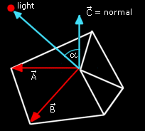
Nothing easier! The final value will have a value in the range 0.0 - 1.0 and can therefore be easily used to color our polygon (it can be used for example as a factor).
FLAT SHADING
If we apply this procedure on every polygon, we have illuminated the scene in a particular method called FLAT SHADING. Today this method is not used anymore because it doesn't represent objects in a realistic way, every polygon is given a uniform shading and the differences between the colors of adjacent polygons are much too visible.
GOURAUD SHADING
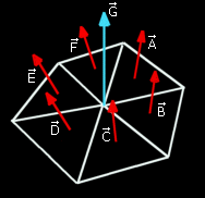
A more realistic but more expensive technique is the GOURAUD SHADING also called SMOOTH SHADING. The main difference of this technique is that instead of using the polygons, normals are used as the vertices normals.
To tell the truth a vertex's normal is a definition that doesn't make much sense! In fact we need a plane to calculate a normal vector!
The correct definition could be instead "Average of the normals of the polygons adjacent to the vertex". Then to calculate a vertex's normal it is enough to make the arithmetic average of the normals of the polygons adjacent to the vertex.
Once you have calculated the vertices normals the procedure for the calculation of the illumination coefficient is the same, nevertheless this time every polygon will have three illumination coefficients, not more only one.
How can we use three coefficients? Simple, when we draw the polygon we apply the illumination using a linear interpolation of the coefficient values to the extreme points of every scan line. The result is an illumination with gradual variations, much more realistic.
And now I have to confess something: we will only have to calculate the normals of the vertices of our object, OpenGL will perform the rest of the job drawing the scene in GOURAUD SHADING! So why don't you take a rest now? ;-)
NORMALS CALCULATION
In this paragraph we will program a function able to calculate all the normals of the vertices in a 3d object. We will do this calculation only once during the initialization phase, during the rendering phase we will pass this data to OpenGL.
To make the code easier to understand we need to create a new file object.c and the relative header in which to store all the object's functions. At first we add (in our object structure, in object.h) an array to contain all the normals of its vertices:
vertex_type normal[MAX_VERTICES];
We open the file object.c and let's write...
void ObjCalcNormals(obj_type_ptr p_object)
{
Let's create some "support" variables...
   int i;
   p3d_type l_vect1,l_vect2,l_vect3,l_vect_b1,l_vect_b2,l_normal;
   int l_connections_qty[MAX_VERTICES];
...and reset all the normals of the vertices
   for (i=0; i<p_object->vertices_qty; i++)
   {
      p_object->normal[i].x = 0.0;
      p_object->normal[i].y = 0.0;
      p_object->normal[i].z = 0.0;
      l_connections_qty[i]=0;
   }
For each polygon...
   for (i=0; i<p_object->polygons_qty; i++)
   {
      l_vect1.x = p_object->vertex[p_object->polygon[i].a].x;
      l_vect1.y = p_object->vertex[p_object->polygon[i].a].y;
      l_vect1.z = p_object->vertex[p_object->polygon[i].a].z;
      l_vect2.x = p_object->vertex[p_object->polygon[i].b].x;
      l_vect2.y = p_object->vertex[p_object->polygon[i].b].y;
      l_vect2.z = p_object->vertex[p_object->polygon[i].b].z;
      l_vect3.x = p_object->vertex[p_object->polygon[i].c].x;
      l_vect3.y = p_object->vertex[p_object->polygon[i].c].y;
      l_vect3.z = p_object->vertex[p_object->polygon[i].c].z;
We create two co-planar vectors using two sides of the polygon:
      VectCreate (&l_vect1, &l_vect2, &l_vect_b1);
      VectCreate (&l_vect1, &l_vect3, &l_vect_b2);
calculate the vector product between these vectors:
VectDotProduct (&l_vect_b1, &l_vect_b2, &l_normal);
and normalize the resulting vector, this is the polygon normal:
VectNormalize (&l_normal);
For each vertex shared by this polygon we increase the number of connections...
      l_connections_qty[p_object->polygon[i].a]+=1;
      l_connections_qty[p_object->polygon[i].b]+=1;
      l_connections_qty[p_object->polygon[i].c]+=1;
... and add the polygon normal:
      p_object->normal[p_object->polygon[i].a].x+=l_normal.x;
      p_object->normal[p_object->polygon[i].a].y+=l_normal.y;
      p_object->normal[p_object->polygon[i].a].z+=l_normal.z;
      p_object->normal[p_object->polygon[i].b].x+=l_normal.x;
      p_object->normal[p_object->polygon[i].b].y+=l_normal.y;
      p_object->normal[p_object->polygon[i].b].z+=l_normal.z;
      p_object->normal[p_object->polygon[i].c].x+=l_normal.x;
      p_object->normal[p_object->polygon[i].c].y+=l_normal.y;
      p_object->normal[p_object->polygon[i].c].z+=l_normal.z;
   }
Now, let's average the polygons normals to obtain the vertices normals!
   for (i=0; i<p_object->vertices_qty; i++)
   {
      if (l_connections_qty[i]>0)
      {
         p_object->normal[i].x /= l_connections_qty[i];
         p_object->normal[i].y /= l_connections_qty[i];
         p_object->normal[i].z /= l_connections_qty[i];
      }
   }
}
In the file object.c we insert also another function that allows to initialize every aspect of the object:
char ObjLoad(char *p_object_name, char *p_texture_name)
{
   if (Load3DS (&object,p_object_name)==0) return(0);
   object.id_texture=LoadBMP(p_texture_name);
   ObjCalcNormals(&object);
   return (1);
}
AND NOW LET'S DRAW THE ILLUMINATED WORLD
The last change to make concerns the drawing routine. We must send to OpenGL the normals of the object. The OpenGL function that does this is glNormal3f.
- void glNormal3f( GLfloat nx, GLfloat ny, GLfloat nz ); specifies the three coordinates x, y, z of the current normal.
Here is the new drawing routine:
glBegin(GL_TRIANGLES);
   for (j=0;j<object.polygons_qty;j++)
   {
      //----------------- FIRST VERTEX -----------------
      //Normal coordinates of the first vertex
      glNormal3f( object.normal[ object.polygon[j].a ].x,
                  object.normal[ object.polygon[j].a ].y,
                  object.normal[ object.polygon[j].a ].z);
      // Texture coordinates of the first vertex
      glTexCoord2f( object.mapcoord[ object.polygon[j].a ].u,
                    object.mapcoord[ object.polygon[j].a ].v);
      // Coordinates of the first vertex
      glVertex3f( object.vertex[ object.polygon[j].a ].x,
                  object.vertex[ object.polygon[j].a ].y,
                  object.vertex[ object.polygon[j].a ].z);

      //----------------- SECOND VERTEX -----------------
      //Normal coordinates of the second vertex
      glNormal3f( object.normal[ object.polygon[j].b ].x,
                  object.normal[ object.polygon[j].b ].y,
                  object.normal[ object.polygon[j].b ].z);
      // Texture coordinates of the second vertex
      glTexCoord2f( object.mapcoord[ object.polygon[j].b ].u,
                    object.mapcoord[ object.polygon[j].b ].v);
      // Coordinates of the second vertex
      glVertex3f( object.vertex[ object.polygon[j].b ].x,
                  object.vertex[ object.polygon[j].b ].y,
                  object.vertex[ object.polygon[j].b ].z);

      //----------------- THIRD VERTEX -----------------
      //Normal coordinates of the third vertex
      glNormal3f( object.normal[ object.polygon[j].c ].x,
                  object.normal[ object.polygon[j].c ].y,
                  object.normal[ object.polygon[j].c ].z);
      // Texture coordinates of the third vertex
      glTexCoord2f( object.mapcoord[ object.polygon[j].c ].u,
                    object.mapcoord[ object.polygon[j].c ].v);
      // Coordinates of the Third vertex
      glVertex3f( object.vertex[ object.polygon[j].c ].x,
                  object.vertex[ object.polygon[j].c ].y,
                  object.vertex[ object.polygon[j].c ].z);
   }
glEnd();
CONCLUSIONS
Finally we have reached the end, and we have survived, hopefully! This was a very technical tutorial, but we have learned some very important theory. The notions studied here will certainly be useful for the next tutorial in which we will introduce matrices. Matrices will allow us to manage the position and the orientation of the objects.
Are you tired of the random rotation of your spaceship? ;-)
SOURCE CODE
The Source Code of this lesson can be downloaded from the Tutorials Main Page